In a previous post, I presented
information about the growth of Unicode in terms of the number of
codepoints assigned in each version. The data was displayed as text tables
using the PrettyTable package. As we are visual beings, I think it would be useful
to also present that data using charts. Here I use matplotlib and the same
data sets to produce such visualizations.
Prerequisites
Recall the lists of lists we produced: DA_codepoint_totals, DA_char_totals, and DA_other_totals:
** Growth of codepoints by version: **
[['1.1', 33979, 33979],
 ['2.0', 144521, 178500],
 ['2.1', 2, 178502],
 ['3.0', 10307, 188809],
 ['3.1', 44978, 233787],
 ['3.2', 1016, 234803],
 ['4.0', 1226, 236029],
 ['4.1', 1273, 237302],
 ['5.0', 1369, 238671],
 ['5.1', 1624, 240295],
 ['5.2', 6648, 246943],
 ['6.0', 2088, 249031],
 ['6.1', 732, 249763],
 ['6.2', 1, 249764],
 ['6.3', 5, 249769],
 ['7.0', 2834, 252603],
 ['8.0', 7716, 260319],
 ['9.0', 7500, 267819]]
** Growth of characters per version: **
[['1.1', 27512, 27512],
 ['2.0', 11373, 38885],
 ['2.1', 2, 38887],
 ['3.0', 10307, 49194],
 ['3.1', 44946, 94140],
 ['3.2', 1016, 95156],
 ['4.0', 1226, 96382],
 ['4.1', 1273, 97655],
 ['5.0', 1369, 99024],
 ['5.1', 1624, 100648],
 ['5.2', 6648, 107296],
 ['6.0', 2088, 109384],
 ['6.1', 732, 110116],
 ['6.2', 1, 110117],
 ['6.3', 5, 110122],
 ['7.0', 2834, 112956],
 ['8.0', 7716, 120672],
 ['9.0', 7500, 128172]]
** Growth of noncharacters per version: **
[['1.1', 6467, 6467],
 ['2.0', 133148, 139615],
 ['2.1', 0, 139615],
 ['3.0', 0, 139615],
 ['3.1', 32, 139647],
 ['3.2', 0, 139647],
 ['4.0', 0, 139647],
 ['4.1', 0, 139647],
 ['5.0', 0, 139647],
 ['5.1', 0, 139647],
 ['5.2', 0, 139647],
 ['6.0', 0, 139647],
 ['6.1', 0, 139647],
 ['6.2', 0, 139647],
 ['6.3', 0, 139647],
 ['7.0', 0, 139647],
 ['8.0', 0, 139647],
 ['9.0', 0, 139647]]
Approach
Import the Python modules needed for this task:
import matplotlib.pyplot as plt
import matplotlib.ticker as ticker
Use Jupyter magic to show plots within the notebook:
Plot line graphs
The x axis is the arange of the number of versions, not the version number itself. The y axis is the number of characters get values for x and y axes. Convert list of lists to numpy array, then read columms from array into lists: x values from column 0, y values from column 2. Use numpy slice [:,0] to read the matrix by column. Convert y values to type int when slicing.
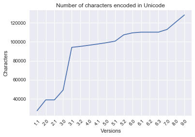
Line graph: number of characters per version
char_array = np.array(DA_char_totals)
fig, ax = plt.subplots()

plt.title('Number of characters encoded in Unicode')
plt.ylabel('Characters')
plt.xlabel('Versions')

x_values = char_array[:,0]
x_range = np.arange(len(x_values))
y_values = char_array[:,2].astype(int)

ax.set_xticks(x_range)
ax.set_xticklabels(x_values, rotation=45)

ax.plot (x_range, y_values)
[<matplotlib.lines.Line2D at 0x973c610>]
As we will be plotting two more graphs of the same type and using the same type of container, it is practical to create a function for the above plot type:
def plot_line_graph(list_, labels_):

    # process parameters

    char_array = np.array(list_)

    plt_title, plt_ylabel, plt_xlabel = labels_

    # set up plot

    fig, ax = plt.subplots()

    plt.title(plt_title)
    plt.ylabel(plt_ylabel)
    plt.xlabel(plt_xlabel)

    x_values = char_array[:,0]
    x_range = np.arange(len(x_values))
    y_values = char_array[:,2].astype(int)

    ax.set_xticks(x_range)
    ax.set_xticklabels(x_values, rotation=45)

    ax.plot (x_range, y_values)
Now we can pass a container and a list of labels to the function to generate additional plots:
labels = ['Number of characters encoded in Unicode', 'Characters', 'Versions']
plot_line_graph(DA_char_totals, labels)

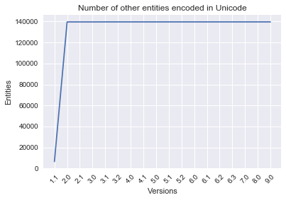
Line graph: number of other entities per version
labels = ['Number of other entities encoded in Unicode', 'Entities', 'Versions']
plot_line_graph(DA_other_totals, labels)
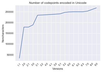
Line graph: number of codepoints assigned per version
labels = ['Number of codepoints encoded in Unicode', 'Noncharacters', 'Versions']
plot_line_graph(DA_codepoint_totals, labels)
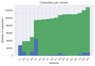
Plot stacked bar graphs
We can also plot the growth of number of characters using a stacked bar graph. Each bar is segmented into smaller categories in order to convey the smaller units that constitute the whole value.
The x axis is the arange of the number of versions, not the version number itself. We will display the actual version numbers by modifying the labels of the plot. Our stacked bar requires two y values: the first (bottom) is the number of new characters per version, the second (top) is the value from the previous version, or, the difference between the total characters for a given version minus the new characters added.
We’ll convert a list of lists to a numpy array, then read columms from the array into lists using numpy slice, eg. [:,0].
Bar graph: growth of number of characters per version
char_array = np.array(DA_char_totals)
Get the difference between the total characters and the new characters for each version. This is expressed as follows:
diff_array = char_array[:,2].astype(int) - char_array[:,1].astype(int)
Set up the plot:
fig, ax = plt.subplots()
ax = plt.axes()

ax.set_title('Characters per version')
ax.set_ylabel('Number of characters')
ax.set_xlabel('Versions')

x_values = char_array[:,0]
x_range = np.arange(len(x_values))

y1_values = char_array[:,1].astype(int)
y2_values = diff_array

y_total = char_array[:,2].astype(int)

ax.xaxis.set_major_locator(ticker.FixedLocator(x_range))
ax.xaxis.set_major_formatter(ticker.FixedFormatter(x_values))
ax.set_xticklabels(x_values, rotation=45)

ax.bar(x_range, y1_values, width=1, label = 'New chars')
ax.bar(x_range, y2_values, width=1, bottom=y1_values, label = 'Total chars')
Commentary
This exercise helped us to convert our data from lists into graphs using matplotlib. The text tables I produced in the previous
exercise, but the visualizations give us another perspective
into the growth of Unicode.